TimescaleDB - Part 1

Time series data is all around us – from financial data to the Internet of Things. No matter what field you are working in, time is a significant factor in better understanding your data. Handling billions of rows of such data can become tiresome. So why not make your life easier and try TimescaleDB? Those were our exact thoughts when we decided to experiment with a new database and see if it could meet our needs. In this two-series blog, we will explore TimescaleDB and what it has to offer (part one) and then we will share the results of our experiments as well as some tips and tricks that we have picked up along the way (part two). So, let’s dive into it. 

TimescaleDB is a relational database specialised for working with time series data. It is implemented as a PostgreSQL extension and offers a new way of handling time series data, new functions for time series data analysis and a special way of storing time series data in order to optimise querying such data. 

The main concepts to grasp when starting with TimescaleDB are hypertables. From a user point of view, hypertables look like simple singular tables, but they are, in fact, much more – an abstraction (or more precisely a virtual view) of many smaller, regular PostgreSQL tables called chunks. Each chunk is defined by a time range and only contains data that falls within that range. When a new record is inserted into a hypertable, one of the following two things happens in the background: 

• If the chunk with the appropriate time range already exists, the record is simply inserted in that chunk 
• Otherwise, if the chunk does not yet exist, it is first created and then the record is inserted into it 

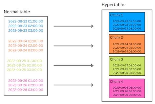
For example, let’s say we have a hypertable with a chunk_interval set to 1 day – meaning each chunk corresponds to one day. In that case, we will have a situation as shown in the picture below, all rows for the 23rd of September will go to one chunk, all rows for the 24th of September to another, and so on. If then a new row comes for the 27th of September, a new chunk for this date will be created as it does not yet exist and the row will be inserted into it. 

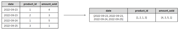
The amount of time series data can grow very quickly so TimescaleDB enables us to save some disk space and potentially speed up certain queries through the use of compression. By setting a compression policy for a hypertable, we call tell TimescaleDB to automatically compress all chunks that are older than a specified time period. Data stored in multiple rows is then converted into a single row in an array format, as seen in the example in the picture below. 

When using compression, it is important to keep in mind what kind of queries we are going to be using the most on our data. Generally speaking, queries on newly ingested data usually cover a smaller time period and cover a bigger number of columns. For this kind of queries, uncompressed data is more suitable to achieve a better query performance. On the other hand, when querying older data, the queries are more analytical in nature and cover a wider time range, but a smaller number of columns. In this case, compressed data results in better query performance. For these reasons, it is important to carefully choose the compression policy interval. 

Sometimes we also do not need to keep all the historical data forever, as it becomes less useful with time, and would benefit from freeing up some extra storage space. Using TimescaleDB’s data retention policy, we can define for how long we want to keep the data in our hypertable before dropping it or we can manually drop data by chunk. 

Very often, we not only want to analyse the raw time-series data but also want to conduct some aggregations on top of our data. But, as the volume of data grows, aggregating on demand can become very slow, especially if you have aggregations you want to run periodically. So, in order to solve that problem, TimescaleDB introduces continuous aggregates. Instead of having to scan the entire table each time the aggregation is run, continuous aggregate already contains the pre-aggregated data and combines it with the most recent data that might not have been included in the aggregation yet to get the final result. The aggregated data in the continuous aggregate is automatically periodically refreshed in the background but can also be refreshed manually when needed. 

Here is an example of creating a continuous aggregate: 

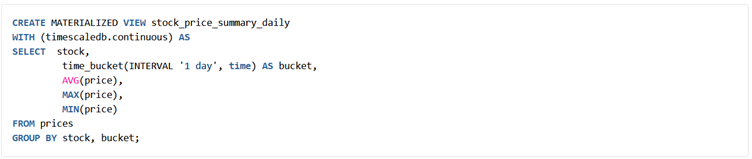
From the example, we can see two things. The first one is that TimescaleDB uses the concept of materialized views to implement continuous aggregates. The second one is the use of the time_bucket function which allows us to group data into time intervals of minutes, hours, etc. 

We can also specify how often we want the data in the continuous aggregate to be refreshed by setting a refresh policy: 

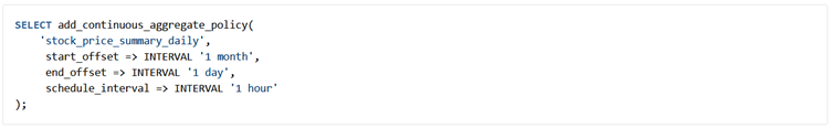
To define a refresh policy, we need to set three parameters: 

• start_offset – the beginning of the refresh window relative to the start of the refresh 
• end_offset – the end of the refresh window relative to the start of the refresh 
• schedule_interval – how often the refreshing is done (set in minutes or hours) 

TimescaleDB also provides useful additional functions that can not be found in the native PostgreSQL to help with the analytical queries. One of them was already mentioned in the context of creating continuous aggregates – time_bucket. Some of the other functions are: 

• first() and last() 

These functions allow you to calculate the first or last values of a column, when ordered by another column (usually time). 

For example, to get the first and last stock price for every stock ordered by time: 

• histogram() 

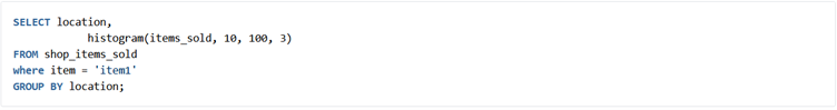
The histogram function allows you to generate a histogram of your data. You need to specify the set of values you want to create a histogram of, the histogram’s lower (inclusive) and upper (exclusive) bound and the number of groups you want to split your data into. The resulting histogram will also have two additional groups: one for all the values that are lower than the lower bound, and one for all the values that are greater than or equal to the upper bound. 

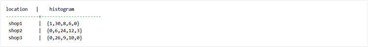
For example, to get the histogram of the number of sold items by the shop location: 

Result:

Congratulations, by this point you have learned the basics of TimescaleDB. Of course, we have only just scratched the surface as TimescaleDB provides many more capabilities. You can refer to the official documentation for more details. And if this blog has drawn your interest, stay tuned for the second one to see TimescaleDB in action. 

Literature: https://docs.timescale.com/