Given that we weren’t really satisfied with the SCD2 implementation inside Airbyte which we explored in our previous blog, we decided to build our own using Python. So, we’re going to give you an overview of how we implemented SCD2 in Python, as well as how the whole pipeline looks. But, before we get into that, let’s look at the data we’re working with.
Data and pipeline
Our dataset is made up of 2 entities: user and user_trx. Their relationship is defined as follows:
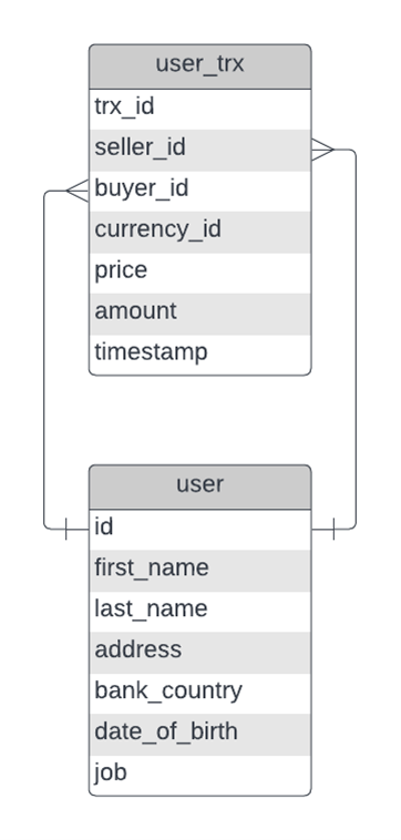
Figure 1. Entity relationship model
A single user can have multiple transactions and can be either a seller or a buyer, but never both simultaneously. Our case required a way to track changes to each seller’s and each buyer’s address and jobs. So, what we did was we split the user_trx into 2 tables representing a seller or a buyer and joined those with the user table to get all the information in a single place. The 2 tables then look as follows:
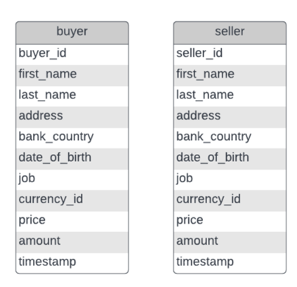
Figure 2. Buyer and seller tables
The process in charge of handling this transformation is called double entry bookkeeping transformation marked at 2) in the figure below. For simplicity, some columns will be hidden in the following examples.
We use Airflow to schedule and orchestrate our whole ETL pipeline, from transferring the dataset to S3, transforming it, and applying SCD2 and finally storing it. The resulting pipeline looks as follows:
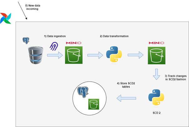
Figure 3. SCD2 ETL process using Python
Step 0 is a process which streams real time user and user_trx data to Postgres. Every day at midnight Airflow triggers our DAG (our pipeline) to process all the data that was streamed to Postgres. The first task is an Airbyte process transferring user and user_trx tables from Postgres. This is done using the AirbyteOperator inside Airflow which precedes the transformation and SCD2 operations. The transformation part creates buyer and seller files which are stored in S3 as temporary files. Once the 2 files are created, the SCD2 process is then started.
Let’s explain the SCD2 process with the buyer entity.
SCD2
Slowly changing dimension (shortly SCD) is a concept used in DWH which enables historical aspects of tracking data. This is an important concept, as many businesses need to keep track of their data, both current and historical. There are different types of SCD implementations, each of them tracks (or doesn’t) historical data differently. Here we focus on SCD type 2, which implements history tracking by adding a new row in a table. How is this row added? Well, if it’s a new record, it is simply appended to a table, but if the record in source contains changes, then the new record will be appended to a table and the old one will be marked as non-active with end date changing to mark when the record has been changed.
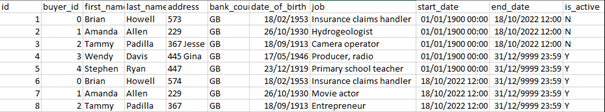
Figure 4. Sample table showing SCD2 records and their corresponding metadata
In the above sample, we can take the buyer_id = 0 example with Brian Howell. Initially, in our target table Brian Howell lived at the 573 address and that was the information we had during our initial load of data. We mark the start_date to an earlier timestamp since it was an initial record, but we could also mark it using the timestamp of the data load or when the change happened (provided we have that information somewhere). 18/10/2022 at 12:00 another data load happened where Brian Howell changed his address to 574. The address column is one of the attributes that we track changes on, so we mark the new record with the new address as active (is_active is set to Y), we set the start_date to mark the data load timestamp (since we don’t have the actual timestamp of the change) and end_date to 31/12/9999. As for the old Brian Howell record, we mark its end_date also to the timestamp of the data load. This way we can chronologically track all the changes that happened to a specific user.
So how did we implement this in Python?
Python SCD2
SCD2 can be logically separated into 3 parts:
- Find and insert new records
- Find and insert changed records
- For every changed record, mark its old value as inactive
We used two types of target destinations, one is an S3 bucket, while the other is a Postgres database. Even though the framework is generic, internally the code is different in order to use the advantage of SQL if we are outputting to a database with the main difference being that we can store the new and changed records to the database without keeping it in memory.
So how exactly did we go about this and what are the input parameters for an SCD2 process?
To capture data change, the source table is left joined to the target table. Naturally, we need to join the tables on some attributes, preferably keys or ids that uniquely identify an object. Those attributes are the first input in our program defined inside a YAML configuration file like this:
KEYS: ["buyer_id", "amount", "currency_id", "price", "timestamp"]
Left join is done by using the Pandas function merge to join the datasets based on given attributes. We additionally add suffixes to differentiate columns coming from the source and columns coming from the target:
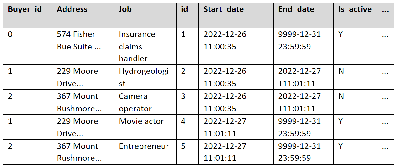
left_df = source_df.merge(dim_curr_df, how='left', on=keys, suffixes=("_src", "_tgt") )One thing to note is, we don’t need to join the whole target table, we only need to join the ones that are currently marked as active records. So e.g., left join from source to target looks something like this (some columns are removed in order to simplify the process and the addresses are fake):
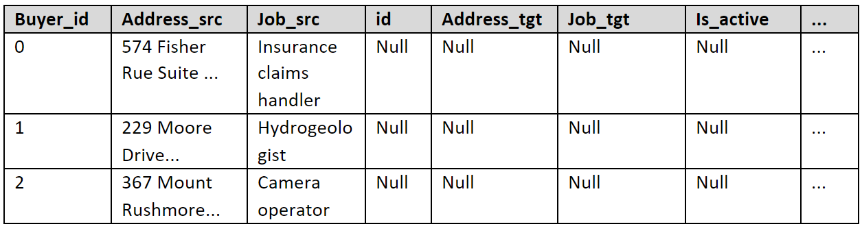
These are all new records because all the attributes with _tgt suffix are NULL. We simply change the values in columns start_date to current processing time (or and timestamp in the past in some cases), end_date to 9999-12-31 23:59:59 and column is_active to ‘Y’. These columns should already exist in our target table (also called a dimension) so there’s no need to recreate them, but we do drop all _tgt columns.
When searching for new records, all the attributes on the right side should be NULL (in our example, attributes with _tgt). Luckily for us, a simple check whether the sequential key is NULL will suffice (which in our case is simply named id). Then, we drop the target columns and rename others if necessary to fit our target column names:
new_df = left_df[left_df[sequence_key].isnull()]new_df = new_df[[col for col in new_df.columns if col[:].endswith("_src") or col in unique_keys] ]new_df.columns = new_df.columns.str.replace("_src", "")new_df["start_date"] = datetime.strptime("1900-01-01 00:00:00", "%Y-%m-%d %H:%M:%S").strftime("%Y-%m-%d %H:%M:%S")new_df["end_date"] = datetime.strptime("9999-12-31 23:59:59", "%Y-%m-%d %H:%M:%S").strftime("%Y-%m-%d %H:%M:%S")new_df["is_active"] = 'Y'
The next step is to figure out which records have changed, and we use another parameter that defines the list of attributes we wish to track changes on, which in our case is only the address:
DIFF_COLS: ['address', 'job']
So, we compare each of the attributes in the list and additionally check whether the sequential key is not NULL:
#Write a dynamic query to compare each source and target column defined in diff_colsquery = f"{sequence_key}.notnull() & ({''.join([col + '_src != ' + col + '_tgt' + ' | ' for col in diff_cols])}"query = query.rsplit("|", 1)[0] + ")"changed_df = left_df.query(query)changed_df = changed_df[changed_df.columns.drop(list(changed_df.filter(regex="_tgt")))]changed_df["start_date"] = kwargs["start_date"] # Start date of the processchanged_df["is_active"] = 'Y'changed_df.columns = changed_df.columns.str.replace("_src", "")changed_df = changed_df.drop("id", axis=1)
After such filtering we get a new dataset reflecting only the changes on the source, e.g.:
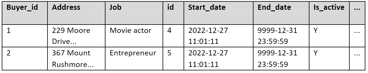
The two changed records have different jobs from before and are marked as currently active records then. The older records will be marked as not active with ‘N’ flag. We can do this in Pandas like this:
# Filter active recordsdim_curr_df = dim_df[(dim_df["is_active"] == 'Y')]# Filter non active recordsdim_non_curr_df = dim_df[(dim_df["is_active"] == 'N')]...concat_df = pd.concat([dim_curr_df, changed_df], ignore_index=True)# only the last record isn't a duplicate, meaning we set end_date to the start # of the changed recordconcat_df["duplicate"] = concat_df.duplicated(subset=keys, keep='last')concat_df["end_date"] = np.where((concat_df["duplicate"] == True) & (concat_df["end_date"] == "9999-12-31 23:59:59"), kwargs[“start_date”], concat_df["end_date"])concat_df["is_active"] = np.where(concat_df["end_date"] != "9999-12-31 23:59:59", 'N', 'Y')concat_df = concat_df.drop("duplicate", axis=1)#Concatenate all the dataframes to get full record historyconcat_df = pd.concat([concat_df, new_df], ignore_index=True)concat_df = pd.concat([dim_non_curr_df, concat_df], ignore_index=True)
After all that, our results look something like this:
One thing to mention is, we are not tracking deletes on source, mostly because they rarely (or shouldn’t even) happen, and our case doesn’t require it.
Let’s look at how we automated this process using Apache Airflow.
Airflow SCD2 S3 -> Postgres
We use Airflow to schedule and orchestrate our tasks and DAGs (Directed Acyclic Graphs). It is not a UI tool per se, because in order to write a DAG we need to write Python code. Once we defined our DAG, we can view it inside the UI:
![]()
This is our DAG view on the homepage where we can see the name of our DAG, its owner, number of runs, trigger rule, last run timestamp and some other options too. We can enable/disable a DAG using the toggle button on the left. Once a DAG is enabled, it will run based on the defined schedule.
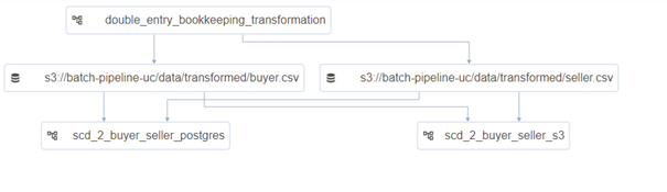
Essentially, inside our DAG we will simply use our Python SCD2 framework, with a few configured parameters for our specific needs, to do all the heavy lifting. Each DAG in Airflow represents a set of tasks that either run sequentially or concurrently and is represented as a graph:
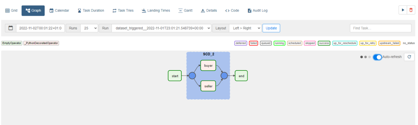
This DAG represents the SCD2 transformation for 2 datasets: buyer and seller. The datasets contain information about a user such as first and last name, address, phone number, amount of crypto sold or bought, type of crypto used in a transaction, pseudonym of the person and their favorite crypto currency. We are mostly interested in tracking the user’s pseudonym and address changes. The only difference in the 2 tasks is the different configuration parameters. This DAG does not have a strict schedule it needs to run on, but rather it waits for certain datasets to be updated on S3, and only then is the DAG triggered. This is a cool feature introduced in Airflow 2.4 called Data aware scheduling. Once the DAG is run, the 2 datasets are taken from S3, put through our SCD2 pipeline and finally transferred to a Postgres table. The start and end tasks are empty operators that do nothing, they are simply here to unify the DAG with a start point and an end point.
Airflow provides a functionality to display DAGs in various ways, for e.g., Grid view:
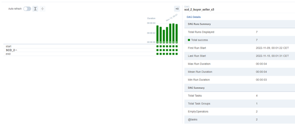
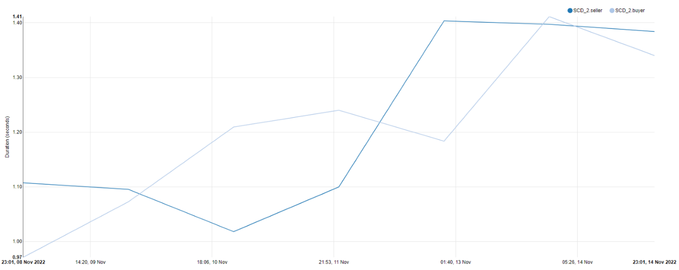
We can also view the logs of each task, the DAG code itself or even task duration view:
Airflow SCD2 S3 -> S3
The DAG pipeline S3 -> S3 looks completely the same as the one above, at least superficially. Internally, as mentioned, the code is handled differently, and the outputs are of course different. The major difference in how the transformation is handled is due to having no intermediate persistence of data, meaning the whole dataset is kept in memory during the execution of the process.
Though this is the end of our process, we’ve mentioned already that it is triggered upon update of certain datasets. So, let’s explain that part a little bit.
Data aware scheduling
The SCD2 process is the final process of our pipeline. The process is triggered when 2 data sources are changed and then we capture those changes. The upstream process splits a single dataset into 2 datasets that are then used in the SCD2 process. Overall, the DAG and dataset dependencies look as follows:
In order to initialize such scheduling, we need to define one or more datasets inside both the DAG that “produces” the dataset and the DAG that “consumes” the dataset. In the producer DAG, we set the outlets parameter to point to the datasets defined, while in the consumer DAG, we set the schedule parameter to point to the datasets the producer produces or changes.
Security
Since we are using S3 as the source and S3/Postgres as the destination, a question that arises is how we can store credentials. Python doesn’t come with something like a keystore and saving it as an environment variable might not be the best possible solution. Luckily, Airflow comes with its own Connections functionality allowing us to store credentials for lots of other services:
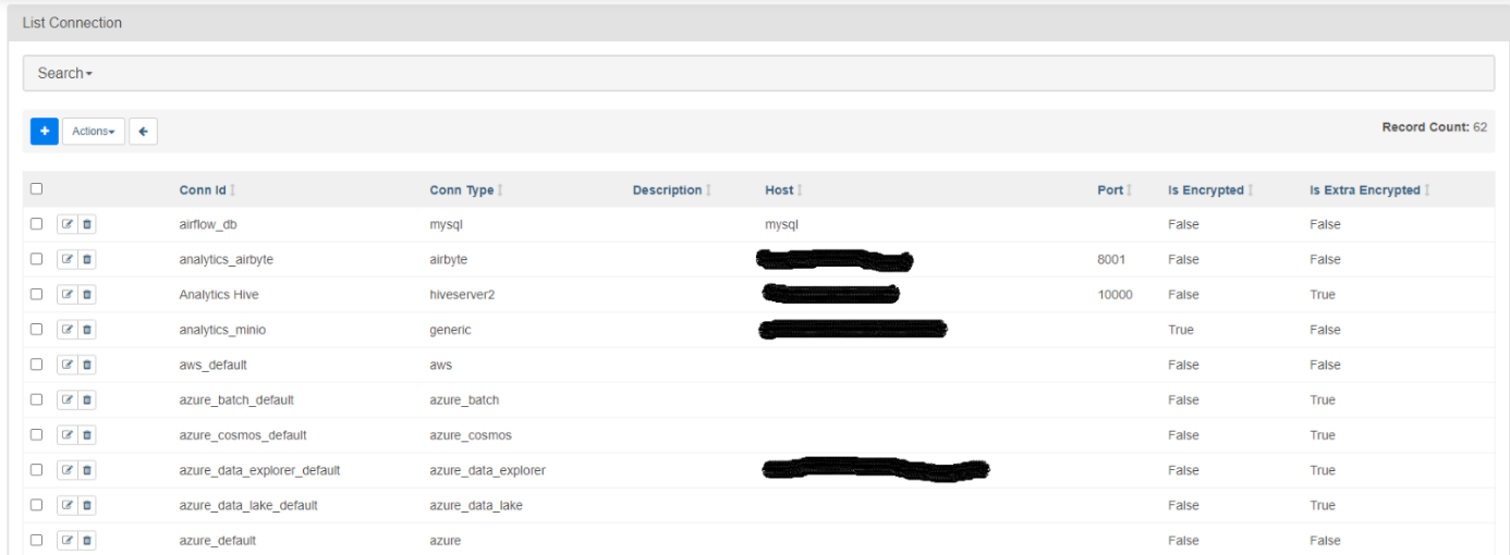
We can add or edit an existing connection, e.g.:
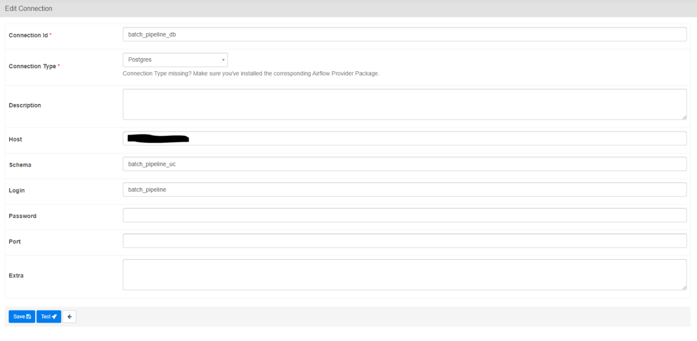
The passwords are not visible in the UI, nor in logging, so it’s out of plain sight. We can fetch the connection inside the execution of our DAG and simply pass the parameter to our code.
Conclusion
Python is used more and more as an ETL tool and one of our needs was to specifically build an SCD2 pipeline. There are already other tools to make SCD2 generic such as SQL Server Management Studio, so there was obviously a way to create generic methods in Python too. We then used Airflow in order to connect the whole pipeline and schedule it as we see fit.
In our next blog, we will introduce dbt and how we managed to integrate it with Airbyte and Airflow!
Data blog series (3 of 5):
Pt.1 – Modern ETL/ELT
Pt. 2 – EL(T) with Airbyte
Pt. 3 – Python generic SCD2 framework
Pt. 4 – Introduction to dbt