In the previous blog post, we introduced the concept of ELT and how it gained popularity lately with modern data systems. In this blog post we will introduce Airbyte, one of the most popular EL(T) tools today. 

Simply put, Airbyte is a tool that makes it easier for you to setup data loads in a matter of minutes. Just with that functionality, it brings a lot of value to the table, but Airbyte offers much more than that. It can be considered as a data pipelines platform. It is an open-source tool, but there is also an Airbyte Cloud commercial offering available in case you want to focus on delivery and forget about infrastructure maintenance. 

Often, you will see Airbyte being mentioned as an EL(T) tool. That is because Airbyte’s basic functionality covers E and L, and for the T part Airbyte natively integrates with dbt (which we will cover in one of our next blog posts). In this post we will focus on EL in Airbyte. 

So, what do we want to achieve with an EL(T) tool? We want to move data from a source system (e.g., S3 bucket) into a target system (e.g., Postgres database) and if needed transform that data once it is loaded into the target system. The first thing we need to do is to connect to source and target systems. Airbyte does that using connectors, which can be either source or destination connectors. List of supported source and destination connections is quite impressive and community is working hard on providing new connectors continuously. It is important to note that source and destination connectors are developed separately, which means if a source connector for one system is available, it doesn’t necessarily mean that destination connector is also available, and vice versa. 

We can breakdown Airbyte pipeline setup in three steps: 

• Creating source 

• Creating destination 
• Setting up connection 

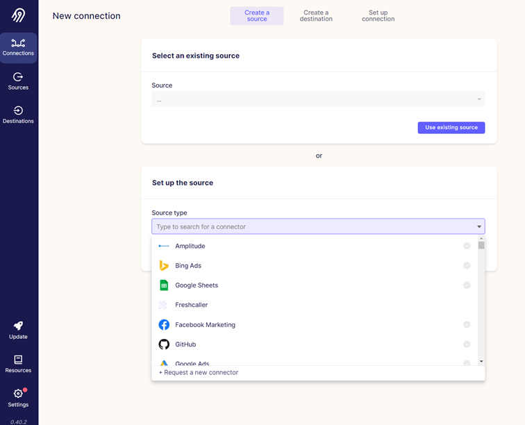
Airbyte UI offers a nice user experience and setting up a new connection is just a couple of clicks away.  

In the remainder of the post, we will demonstrate how we used Airbyte to move data from Postgres to MinIO. 

First, let’s create Postgres source. From the “Source type” dropdown menu, we choose Postgres.  

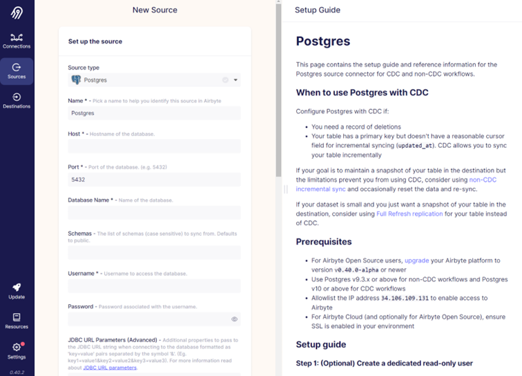
On the right side of the screen there is a setup guide that gives more info on the connector and helps with the setup process.  

Once all the needed information for the new source is entered, Airbyte will test the connection and save it. Now we can move on to setting up a destination. 

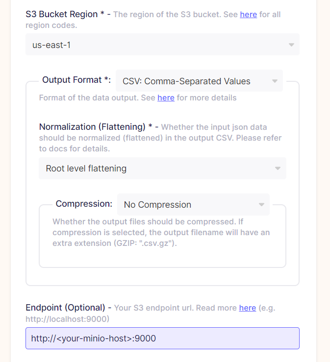
We want to use MinIO as a destination. There is no MinIO connector available, but it is an S3 compatible object store so we can use S3 connector. The process looks very similar to the source setup. 

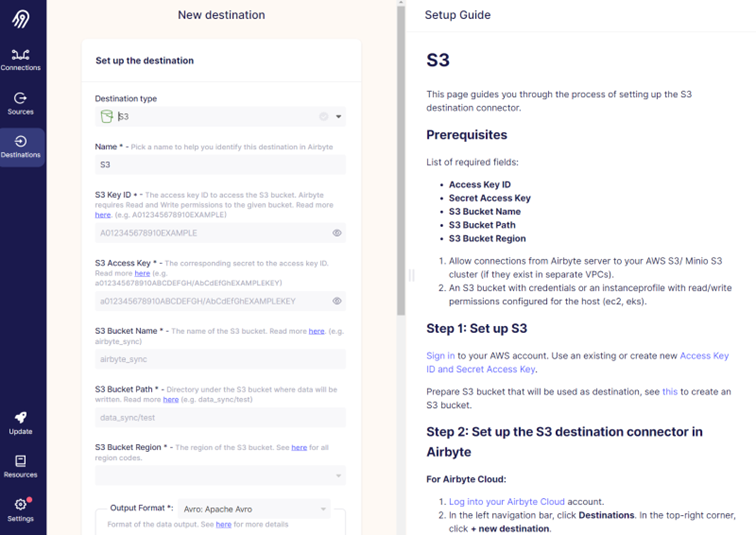
Just to mention a couple of important things since MinIO is used instead of S3. For “S3 Bucket Region”, it is not important what you choose, just pick one since it is a mandatory field. And then in the “Endpoint” field, type in the URL to your MinIO installation. 

We’re almost there! We have a source and destination setup, now we just need to connect them through connection setup. What we basically do in this step is define what objects from source we want to replicate to destination. And what type of replication we want to use.  

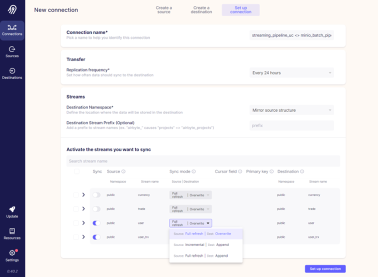
Through Airbyte we can set up how often we want this replication to happen. Every hour, or 24 hours for example. But in our case, we will set it to manual because we will use Airflow for orchestration. 

In our example there are 4 tables in the source database, we will just use two for this example: user and user_trx tables. We won’t go into data here but just for the sake of clarity, table user contains data about users, while user_trx table contains data about users bank card transactions.  

For the sync (or replication) mode, we will use full refresh and overwrite. On the screenshot above you can see that there is also incremental mode available. Sync modes available will depend on the source and destination systems that you are using. And that’s it, all that’s left is to click on “Set up connection” and we are good to go! 

To run data sync, we can open the connection we just created and click on “Sync now” button. 

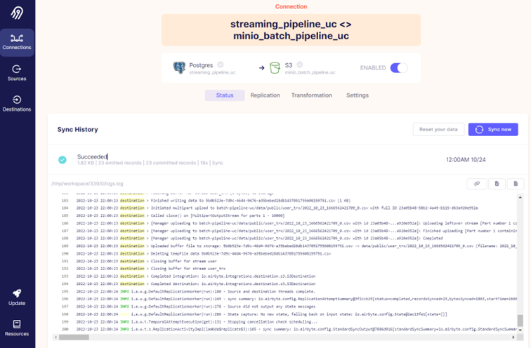
When the sync finishes, we can see the status of sync, how much data was loaded and how long it took. By clicking on the specific sync run we can also see the logs for that run.  

On the connection page you’ll also notice “Transformation” tab where we can define dbt transformations to be applied on the destination. It is important to note that it is not possible to use dbt on all destinations, S3 is one of them.  

As we’ve seen before, there are different sync modes that can be used in Airbyte. With sync mode we define how Airbyte should read data from source and how to write it to our destination. Let’s explain it in a bit more detail. 

There are four possible combinations of source and destination sync mode: 

• Full refresh | Overwrite 
• Full refresh | Append 
• Incremental Sync | Append 
• Incremental Sync | Deduped History

Here are some details about the source part of the sync mode: 

Full refresh

Reads everything from source 

Incremental 

• Reads only increments added to the source since the last sync job
• Depending on the source used there are also two different methods available: 

1. 1. Using a cursor (e.g., incremental column on the source that will be used to detect increments) 

2. Using change data capture (CDC) which is only supported by some sources (e.g., Postgres)

For the destination part we can choose from three options:

Overwrite

• Deletes existing data on the destination and writes new data 

Append 

• Adds data to the existing data in the destination 

Deduped history 

• Append + history

Let’s go into a bit more detail about deduped history sync mode. We’ll do it by comparing it to incremental sync with append mode. One would use incremental sync append mode in situations where there are no deletes or updates happening on the source. For example, that might be the case when handling card transactions data. The source table that holds card transactions data will only have inserts happening on it with each new transaction. But if there were updates and deletes happening on the source, we can use deduped history mode to capture those changes and maintain the same state on the source and destination tables while also keeping track of history. 

With deduped history mode two tables will be maintained on the destination: 

Deduped table 

• Final table that will contain de-duplicated records, I.e., it will hold the current state of data, the same as it is in the source table 

History table 

• Additional table with _scd suffix will contain historical changes of data in SCD2 fashion (we will explain SCD2 in the next paragraph and in the next blog in more details) 
• With that we can quickly look at the current state in the final (deduped) table, or go back in time using history _scd table 

There are just a couple of things that need to be mentioned about SCD2 in history table. Slowly changing dimension (shortly SCD) is a concept used in DWH which enables historical aspects of tracking data. There are different types of SCD implementations, each of them tracks (or doesn’t) historical data differently. Here we focus on SCD type 2, which implements history tracking by adding a new row in a table. 

There are different possible implementations of SCD2. Ralph Kimball, one of the fathers of data warehousing, states his recommendations for SCD2 implementations on this link. 

We like to model our SCD2 tables so that they contain valid_from, valid_to and active_flag columns. Airbyte’s way of modeling SCD2 is somewhat different and we’ll describe those differences in the remainder of this blog. 

Airbyte’s history table doesn’t have active_flag column which will make searching for currently active rows more processing intensive on the database. This is mitigated in Airbyte by using an additional deduped table which holds current state, but at cost of storing more data.  

Another difference between Airbyte’s and our prefered way of modelling SCD2 is that Airbyte’s valid_to value on active record is NULL instead of some distant value in the future (in our case 31/12/9999). Having NULL in valid_to column is not a good practice because NULL can’t be compared in SQL query. So, for example query in which we are looking for values where valid_to is between ‘2020-01-01′ and ‘2022-01-01′ will return “wrong” result.  

We’ve been using Airbyte for quite some time now and we love it. It is an easy to use EL(T) tool that can be run in Docker in no time. It provides a great number of connectors and the list is growing constantly. With different sync modes available, it covers the most important cases you could have with replicating data. The only thing that we would like to change are the SCD2 table modelling bits mentioned above.  

Stay tuned! In the next blog post we will demonstrate how we implemented generic SCD2 framework in Python, and how the entire data flow was orchestrated with Airflow. 

Data blog series (2 of 5):  

Part 1