AI-powered vs. Traditional Search (Vol. 3): Case Study

Let’s continue where we left off in the previous part of this blog series about AI-powered search.

Local AI-powered search application

Now that we’ve explored various AI-powered search techniques and their use cases, let’s dive into a practical example of building a search service that incorporates many of these components. Our goal is to enhance search functionality over an existing document database, using the methods we’ve discussed so far. Furthermore, we aim to have the whole solution deployed and running locally, without relying on any cloud services or models.

The dataset

For our AI-powered search use case, we’ll assume our dataset consists of simple PDF documents, each around 10-15 pages long. Examples of such datasets could include company HR documents, an index of research papers, or a collection of legal case summaries. Let’s assume the documents are already stored in some type of relational database – both as binary files of the original document and text value extracted from the document.

Choosing a storage provider

There are many options when it comes to choosing storage for our use case. Since our documents are already stored in a relational database, we can leverage its capabilities for basic metadata storage and structured queries. However, if we want to leverage more advanced AI-powered search capabilities, such as ranking algorithms, semantic search or RAG, we need to extend our storage solution.

The first option is to use one of the many open-source search engines supporting traditional index-based storage and retrieval. Two examples include Apache Lucene and Apache Solr.

Apache Lucene is a low-level search engine implemented in Java, with library support for various other languages. It supports inverted indexing, full text search and ranking, with excellent performance. However, due to its low-level nature, it needs to be integrated at code level via its API, requiring a decent amount of developer effort to handle indexing, searching and managing the search process. This, however, makes it excellent for embedding into applications where fine-grained control and optimisation of the search process is important.

Apache Solr, on the other hand, is a standalone search server built on top of Lucene, that can be independently deployed and used out-of-the-box. It supports faceted search, distributed search, query caching, and schema management. Its extensive plugin ecosystem further simplifies complex tasks such as indexing rich content formats and detecting document languages.

The second option is to use a dedicated embedding database to store embedded chunks of the original documents, and retrieve them based on the similarity to the embedded query. The important criteria when choosing such a database are its scalability, low-latency search and an API that allows easy insert/retrieval into and from the database. Popular open-source choices include Chroma, Pinecone, Milvus and FAISS.

However, each of these two options has the drawback of supporting only one search approach – either „traditional“ index based search (Apache Lucene and Apache Solr), or embedding search. We want a solution that supports both.

That’s where Elasticsearch and its open-source fork OpenSearch shine. As distributed search engines, they combine the strengths of traditional keyword-based search and embedding-based vector search. Built on top of Apache Lucene, they provide support for full-text search, including BM25 ranking, fuzzy search, faceted filtering and domain-specific languages (DSL) queries – very similar to capabilities provided by Apache Solr.

However, they also provide native support for vector search through aNN, using algorithms such as HNSW, eliminating the need for a separate embedding database in many use cases. Finally, they offer support for hybrid search, allowing the user to combine the power of traditional and embedding search into a single, powerful search experience.

Performance considerations

To be clear, even though Elasticsearch and OpenSearch support vector search and in many use cases act exactly like an embedding database, their primary purpose is indexing textual documents using inverted indexes – support for vector search was added later. This makes optimising the whole architecture for dense vector search difficult.

In contrast, dedicated vector databases like Pinecone, Chroma, or FAISS are specifically designed for high-speed, large-scale vector operations, often resulting in lower computational overhead and faster retrieval times compared to Elasticsearch.

If vector search is your only requirement a dedicated vector database is likely the better choice. However, if you want to support traditional search, as well as hybrid approaches, and you want a solution with easy support for scaling and load balancing, Elasticsearch remains a good choice.

Elasticsearch vs OpenSearch

Elasticsearch and OpenSearch share a common foundation and both offer robust solutions for AI-powered search. OpenSearch was created as an Elasticsearch 7.10 fork after the changes to Elasticsearch’s licensing models. It means they share a lot of their key features, with a couple of differences:

• Both engines support BM25, fuzzy search, embedding search and hybrid search
• Elasticsearch is generally thought to have more mature vector search capabilities, owning to optimizations to the HNSW algorithm. However, the development of both engines is still ongoing, and it is possible OpenSearch catches up at a point
• OpenSearch has an Apache 2.0 license, whereas Elasticsearch uses the more restrictive dual license (SSPL and Elastic License 2.0)
• Elasticsearch contains some proprietary features, including the integrated embedding model ELSER
• Both engines support both local and on-cloud deployment: Elastic Cloud for Elasticsearch and OpenSearch Service on AWS for OpenSearch

In the rest of this tutorial, I’m going to go with Elasticsearch as our storage provider, mainly due to easier integration and better support owing to its longer existence. However, I do encourage you to try out both and compare them for your specific use case.

To ELSER or not to ELSER

When incorporating semantic search into our system, we need to decide how to generate text embeddings. Elasticsearch provides two primary options: using its proprietary ELSER (Elastic Learned Sparse Encoder) model or leveraging a third-party embedding model.

Using ELSER

ELSER (Elastic Learned Sparse EncodeR) is Elastic’s built-in embedding model, designed to enable semantic search without requiring an external embedding pipeline. In other words, you can simply index your data as usual, in textual format, and leave Elastic to handle the rest. ELSER is a sparse embedding model – meaning the embedding vectors it uses, called sparse vectors, are highly dimensional, but with most of the values being 0. Only the values corresponding to specific semantic information are 1.

This structure allows for better integration with Elasticsearch’s native indexing structure, leading to lower storage overhead and faster query processing compared to dense vectors. However, this feature is only available in commercial Elasticsearch versions. Furthermore, ELSER is recommended for English language documents and queries – in the case multilingual support is needed, it is recommended to use the multilingual alternative, the E5 embedding model.

Using a third-party embedding model

Using a third-party embedding model provides several advantages over Elasticsearch’s built-in ELSER model. For example, third-party models typically offer richer semantic understanding, allowing them to capture subtle meanings and context in text, leading to more accurate and relevant search results.

Another important benefit is multilingual support: unlike ELSER, many third-party embedding models such as Cohere Embed v3, OpenAI’s text-embedding-3-large, or open-source options like Sentence-BERT and Universal Sentence Encoder handle multiple languages effectively, making them a good alternative if your dataset is not in English. Also, ELSER embeddings tend to work best with inputs under 512 characters – if you want to store larger chunks, a third-party model is a better option.

Third-party embedding models give you more flexibility and control. Choosing ELSER means committing to Elasticsearch as your primary (vector) database, meaning if you ever decide to switch to a different provider, you’ll need to regenerate your embeddings using a different model, due to ELSER embeddings tight integration with Elasticsearch. By using a third-party model, you’re much more flexible when switching storage providers.

Lastly, from a more practical perspective, ELSER is only available in paid versions of Elasticsearch – if you’re using the free version, you’ll need to generate and fetch embeddings using a third-party embedding model.

Considering these advantages, we choose third-party embedding models as the backbone of our embeddings in the rest of this tutorial.

Starting up Elasticsearch

To get started with Elasticsearch, you have two common deployment options: hosting it locally on your own infrastructure or using a managed cloud service like Elastic Cloud. For the purposes of this tutorial and simple testing, Docker is a simple and straightforward choice. First, create a file named docker-compose.yml with the following content:

version: '3.7'
services:
  elasticsearch:
    build:
      context: elasticsearch/
      args:
        ELASTIC_VERSION: ${ELASTIC_VERSION}
    volumes:
      - ./elasticsearch/config/elasticsearch.yml:/usr/share/elasticsearch/config/elasticsearch.yml:ro,Z
      - elasticsearch:/usr/share/elasticsearch/data:Z
    ports:
      - 9200:9200
      - 9300:9300
    environment:
      node.name: elasticsearch
      ES_JAVA_OPTS: -Xms512m -Xmx512m
      ELASTIC_PASSWORD: ${ELASTIC_PASSWORD:-}
      discovery.type: single-node
    networks:
      - elk
    restart: unless-stopped
  kibana:
    build:
      context: kibana/
      args:
        ELASTIC_VERSION: ${ELASTIC_VERSION}
    volumes:
      - ./kibana/config/kibana.yml:/usr/share/kibana/config/kibana.yml:ro,Z
    ports:
      - 5601:5601
    environment:
      KIBANA_SYSTEM_PASSWORD: ${KIBANA_SYSTEM_PASSWORD:-}
    networks:
      - elk
    depends_on:
      - elasticsearch
    restart: unless-stopped
networks:
  elk:
    driver: bridge
volumes:
  elasticsearch:

Then, from the directory containing this file, run docker-compose up -d. This will launch a single-node Elasticsearch instance accessible at localhost:9200, alongside a Kibana instance on localhost:5601.

Creating the indexes

Before inserting our data, we need to create the indexes where our data will be stored.

For our example use case, we’ll create two indexes:

• info_index
  • contains basic information about the stored documents, such as title, title embedding, authors, abstract and abstract embedding
• content_index
  • contains the content of each document split into chunks and their respective embeddings

We can create the indexes either through the Kibana UI (available on localhost:5601), or through an API request, shown below:

PUT /your-index-name
{
  "mappings": {
    "properties": {
      "abstract": {
        "type": "text",
        "fields": {
          "keyword": {
            "type": "keyword",
            "ignore_above": 256
          }
        }
      },
      "abstract_embedding": {
        "type": "dense_vector",
        "dims": 1024,
        "index": true,
        "similarity": "cosine",
        "index_options": {
          "type": "int8_hnsw",
          "m": 16,
          "ef_construction": 100
        }
      },
      "authors": {
        "type": "text",
        "fields": {
          "keyword": {
            "type": "keyword",
            "ignore_above": 256
          }
        }
      },
      "id": {
        "type": "long"
      },
      "title": {
        "type": "text",
        "fields": {
          "keyword": {
            "type": "keyword",
            "ignore_above": 256
          }
        }
      },
      "title_embedding": {
        "type": "dense_vector",
        "dims": 1024,
        "index": true,
        "similarity": "cosine",
        "index_options": {
          "type": "int8_hnsw",
          "m": 16,
          "ef_construction": 100
        }
      }
    }
  }
}

In a similar manner we can create the content_index.

Take note which fields are of type „text“ and which are of type „dense vector“ – fields of type „text“ are searchable using traditional retrieval methods available in Elasticsearch, while fields with the type „dense vector“ are embedding vectors and support embedding search using vector similarity.

Once we have setup our Elasticsearch and created the necessary indexes, we’re almost ready to insert our data. However, there are two things we need to consider before – the embedding model we’ll use and the way we’ll split our document content text into smaller chunks for embeddings.

Embedding model

As we’re using a third-party embedding model instead of Elasticsearch’s proprietary ELSER, there are plenty of great options to choose from. Probably the most common embedding models today are OpenAI’s embeddings—they’re inexpensive, fast, and generally considered high quality. However, they’re only accessible through a cloud-based API, which doesn’t align with our goal of deploying a fully local search solution. Thus, we need to look elsewhere—and what better place than Hugging Face?

Specifically, we’ll be using the BAAI BGE-M3 embedding model hosted on Hugging Face.

BGE-M3 stands out due to its excellent multilingual support (covering over 100 languages), strong semantic understanding, and impressive performance on retrieval tasks. Additionally, it supports multiple retrieval methods—dense retrieval, sparse retrieval, and multi-vector retrieval—giving us flexibility in how we structure our search pipeline. With a maximum input length of 8192 tokens and embeddings of dimension 1024, it’s well-suited for handling both short queries and longer documents effectively. Finally, as an open-source model licensed under MIT, BGE-M3 fits perfectly with our requirement of running everything locally without licensing constraints.

Following is a simple example of using the model to fetch embeddings for a sample text:

from transformers import AutoTokenizer, AutoModel

import torch # Load the BAAI BGE-M3 model and tokenizer

model_name = "BAAI/bge-m3" tokenizer = AutoTokenizer.from_pretrained(model_name) 
model = AutoModel.from_pretrained(model_name) # Use GPU if available, otherwise fallback to CPU 
device = torch.device('cuda' if torch.cuda.is_available() else 'cpu') 
model.to(device)

 # Function to generate embeddings

def get_embeddings(texts):

    inputs = tokenizer(texts, padding=True, truncation=True,

return_tensors="pt").to(device)

    with torch.no_grad(): # Generate embeddings and return as a list

        embeddings = model(**inputs).last_hidden_state.mean(dim=1).cpu().tolist()

    return embeddings


# Example usage
if __name__ == "__main__":

    sample_texts = ["What is BGE M3?", "Explain dense retrieval."

    embeddings = get_embeddings(sample_texts)

    print("Embeddings:", embeddings)

Chunking

Before embedding our documents, we need to split them into smaller chunks that fit within the maximum input size supported by our embedding model. Although the BAAI BGE-M3 model supports a maximum input length of 8192 tokens, the recommended chunk size for vector search is usually between 512 and 2048 tokens. We opted for the middle and chose 1024 for the size of our chunk, with chunk overlap of 200 tokens. Thus, we need to split our documents with a length of more than 1024 tokens into smaller chunks.

There are a number of different chunking approaches currently in existence, however we focused on two – recursive text splitting and semantic chunking.

Recursive text splitting works by recursively dividing text into chunks of a specified maximum size while attempting to preserve natural boundaries—first splitting by paragraphs (\n\n), then sentences (\n), and finally words ( ). This minimizes disruptions to the semantic flow within each chunk. Additionally, this method supports measuring chunk sizes by tokens rather than characters, allowing us to align directly with the token limit of our embedding model.

While recursive text splitting is probably the most common chunking strategy, a number of other strategies do exist. One new and promising approach is semantic chunking. Instead of relying on fixed delimiters, semantic chunker uses embeddings to evaluate sentence similarity and groups semantically related sentences into coherent chunks. This ensures that context is preserved within each segment, making it particularly valuable for applications like retrieval-augmented generation (RAG) or document retrieval systems where maintaining semantic integrity is critical.

Semantic chunking provides flexibility by allowing developers to customize parameters such as similarity thresholds and chunk sizes to suit specific use cases. It excels in handling large documents and complex queries by focusing on logical split points like paragraph boundaries or thematic sections.

However, it does come with higher computational overhead since it requires embedding models to calculate similarities between sentences or paragraphs, potentially requiring large amounts of VRAM due to the use of the embedding models. While this resource constraints made it impractical for our local deployment, it remains a compelling option for systems with greater computational resources or cloud-based infrastructure.

Inserting data into Elasticsearch

Once the documents are prepared, the next step is inserting them into Elasticsearch for indexing. In this implementation, we use the official Elasticsearch Python SDK (Elasticsearch package), which provides a convenient way to interact with Elasticsearch APIs. You can also use the Elasticsearch REST API if you prefer.

Here’s a basic example of how you can insert a document using the Elasticsearch SDK directly:

from elasticsearch import Elasticsearch
from service.embeddings import embeddings

# Initialize Elasticsearch client
client = Elasticsearch("http://username:password@localhost:9200")

# assuming the paper_title, paper_abstract and other fields have already been initialized
# and assuming embeddings is a service that fetches embeddings given a string object

paper_title_embedding = embeddings.embed_documents([paper_title])[0]
paper_abstract_embedding = embeddings.embed_documents([paper_abstract])[0]

# Define the document body
document_body = {
   'id': paper_id,
   'authors': paper_authors,
   'title': paper_title,
   'title_embedding': paper_title_embedding,
   'abstract': paper_abstract,
   'abstract_embedding': paper_abstract_embedding
}
# Insert the document into the index using a pipeline
response = client.index(index="info_index", id=None, body=document_body, pipeline=None)
print("Document indexed:", response)

In a similar manner we can index the content of the documents we split into chunks using the semantic chunker. Here each chunk is a single document in Elasticsearch, with a reference to the original document for easy retrieval.

# then, split the content into chunks
# add each chunk separately into content index
chunks = recursive_text_splitter.create_documents([paper_content])
chunk_texts = [chunk.page_content for chunk in chunks]
chunk_embeddings = embeddings.embed_documents(chunk_texts)
id = 0
for i in range(len(chunk_texts)):
   chunk_text = chunk_texts[i]
   chunk_embedding = chunk_embeddings[i]
   chunk_id = str(paper_id) + "_" + str(hash(chunk_text))
   chunk_content_data = {
      'id': paper_id,
      'title': paper_title,
      'title_embedding': paper_title_embedding,
      'abstract': paper_abstract,
      'abstract_embedding': paper_abstract_embedding,
      'content_chunk_id': chunk_id,
      'content_text': chunk_text,
      'content_embedding': chunk_embedding
   }
   # add the chunk data as document to content-index
   client.index(index="content_index", id=None, body=chunk_content_data, pipeline=None)

Searching the data using Elasticsearch

Once we’ve inserted the data into our indexes, let’s take a look at how we can search it using Elasticsearch REST API calls.

Traditional search

{
  "query": {
    "match": {
      "title": "Metric Learning"
    }
  },
  "_source": {
    "excludes": ["title_embedding", "abstract_embedding"]
  }
}

In this example we find all matches in the „title“ field that correspond to the query „Metric Learning“. In the background, Elasticsearch tokenizes the query and finds the documents containing these terms using inverted index lookup. Then it ranks them using the BM25 algorithm. Finally, the ‘_source’ field specifies which fields of the found documents should be left out from the result – in this case, we leave out the embedding fields as they provide us with no relevant information while taking quite a bit of space.

Vector search

{
  "size": 10,
  "from": 0,
  "knn": {
    "field": "content_embedding",
    "k": 5,
    "num_candidates": 100,
    "query_vector": [
            0.23643067479133606,
            0.5814058184623718,
            -0.9170772433280945,
            0.00640927953645587,
            ...
        ],
    "filter": {
      "bool": {
        "must": [
          {
            "term": {
              "id": 144
            }
          }
        ],
        "must_not": []
      }
    }
  },
  "aggs": {},
  "_source": {
    "excludes": ["title_embedding", "abstract_embedding", "content_embedding"]
  }
}

Here we can see an example of vector search over the field „content_embedding“. To perform vector search, as we’re not using ELSER but a third-party model, we first have to calculate the embedding for our query using our third-party model -in this case, this embedding vector represents the same query as when using traditional search – „Metric Learning“.  Additionally, we specify a Boolean filter, fetching only results from the document with ID 144 – effectively, we’re trying to find all mentions of the term „Metric Learning“ in the document with ID 144. If we wanted to search over chunks of all documents in our index, we’d simply leave out the filter.

The size parameter controls how many results to return – in this case, it will return up to 10 documents sorted by relevance/distance from the query vector.

Parameter ‘k’ specifies the number of final nearest neighbours to return – in this case, 5. ‘num_candidates’ represents the number of potential matches to retrieve during the initial search – so Elasticsearch will retrieve up to 100 candidates and then select the top 5 based on cosine distance. Candidate retrieval is optimized using an approximate search algorithm like HNSW, while the num_candidates parameter controls the trade-off between accuracy and speed:

• higher num_candidates – more accurate but slower
• lower num_candidates – faster but less accurate.

An important thing to note is even though the API request contains „knn“ as one of the parameters for the search, the search algorithm executed after submitting this request is not in fact kNN – but rather aNN. Elasticsearch finds a num_candidates number of approximate nearest neighbour candidates on each shard using an algorithm such as HNSW. It collects the candidates from each shard and merges them to find the top k result. This trade off means that we aren’t 100% guaranteed to find the true nearest neighbour when we perform the search, but we gain a great increase in the speed of the query.

Exact kNN, one that exhaustively compares every vector embedding to the query vector can also be used in Elasticsearch by specifying a custom similarity score to use when comparing vectors. To learn more about this, check out this.

Hybrid search

Elasticsearch also integrates hybrid search in its search capabilities. It combines traditional BM25 based search with vector similarity search (aNN), gaining the best of both worlds.

It does this by first performing seperate BM25 and vector similarity searches and then combining the results into a single set using a reranking algorithm – typically the reciprocal rank fusion (RRF) algorithm.

An example of such a query can be seen below. Some new parameters that we haven’t seen before include:

• Boost values (0.4 for BM25, 0.6 for kNN) balance the relative importance of each search method
• window_size (10) limits how many top results from each method are considered for reranking
• rank_constant (20) controls how quickly relevance decreases in the RRF formula

{
  "size": 20,
  "query": {
    "bool": {
      "must": [
        {
          "match": {
            "content": {
              "query": "Metric Learning",
              "boost": 0.4
            }
          }
        }
      ]
    }
  },
  "knn": {
    "field": "content_embedding",
    "query_vector": [0.236, 0.581, -0.917, 0.006, ...],
    "k": 5,
    "num_candidates": 100,
    "boost": 0.6
  },
  "rank": {
    "rrf": {
      "window_size": 10,
      "rank_constant": 20
    }
  },
  "_source": {
    "excludes": ["content_embedding"]
  }
}

Choosing and running an LLM

You cannot make pizza without flour, and you cannot build a RAG system without an LLM — arguably the most important component of the system. Probably the most popular LLM today is OpenAI’s ChatGPT model, but since it’s available exclusively through the API, it isn’t something we’ll consider when building our local search service.

Fortunately, since ChatGPT’s release, the open-source LLM landscape has expanded with numerous models — from Meta’s LLaMA models and Google’s Gemma series to underdogs-turned-champions like Deepseek’s R1. It’s nearly impossible to recommend a single model for this use case.

This is partly due to new models being released almost weekly, making suggestions quickly obsolete, and partly due to the hardware you have available to run the model. Even with limited hardware resources, you’re almost guaranteed to find a model you can run (and which performs well!) thanks to optimizations like quantization and distillation. During my testing on dual NVIDIA A30 GPUs, each with 24 GB of VRAM, I was able to run the LLaMA 3 70B-Instruct-Q3_K_M model with a satisfactory token output speed, and I found it performed well for the RAG use case.

Once you’ve selected your open-source LLM, all that’s left is to run it. You can either download the model’s source files and weights and run them directly using PyTorch or use one of the available model hosting services like Ollama or vLLM.

During my testing, I found Ollama easy and intuitive to use. To start Ollama, you can use a Docker Compose file like this one, which configures the model to use the GPU if available:

version: '3.8'
services:
  app:
    build: .
    ports:
      - 8000:8000
      - 5678:5678
    volumes:
      - .:/code
    command: uvicorn src.main:app --host 0.0.0.0 --port 8000 --reload
    restart: always
    depends_on:
      - ollama
      - ollama-webui
    networks:
      - ollama-docker
      
  ollama:
    volumes:
      - ./ollama/ollama:/root/.ollama
    container_name: ollama
    pull_policy: always
    tty: true
    restart: unless-stopped
    image: ollama/ollama:latest
    ports:
      - 7869:11434
    environment:
      - OLLAMA_KEEP_ALIVE=24h
      - OLLAMA_MODELS=/storage/ollama
    networks:
      - ollama-docker
    deploy:
      resources:
        reservations:
          devices:
            - driver: nvidia
              count: 2
              capabilities: [gpu]
  ollama-webui:
    image: ghcr.io/open-webui/open-webui:main
    container_name: ollama-webui
    volumes:
      - ./ollama/ollama-webui:/app/backend/data
      
    depends_on:
      - ollama
    ports:
      - 8080:8080
    environment: # https://docs.openwebui.com/getting-started/env-configuration#default_models
      - OLLAMA_BASE_URLS=http://host.docker.internal:7869 #comma separated ollama hosts
      - ENV=dev
      - WEBUI_AUTH=False
      - WEBUI_NAME=valiantlynx AI
      - WEBUI_URL=http://localhost:8080
      - WEBUI_SECRET_KEY=t0p-s3cr3t
    extra_hosts:
      - host.docker.internal:host-gateway
    restart: unless-stopped
    networks:
      - ollama-docker
networks:
  ollama-docker:
    external: false

Once you’ve ran this docker compose, the Ollama service should be available at two endpoints:
             

• http://localhost:7869/api/generate
  • the endpoint for API requests
• http://locahost:8080/
  • the endpoint for OpenWeb UI, an interactive UI you can use to experiment with your local LLMs

To see all the available models, you can download and use with Ollama, you can go here. You can install your chosen model either through the OpenWeb UI or Ollama command line.

An example Ollama API request might look something like this:

curl http://localhost:11434/api/chat -d '{
  "model": "llama3.3",
  "messages": [
    {"role": "system", "content": "You are a helpful assistant."},
    {"role": "user", "content": "What is the capital of France?"}
  ],
  "stream": false
}'

Full Ollama API specification is available at this link. The API supports all the usual features, such as streaming, function calling, structured outputs etc.

Refining Relevance with Reranking

While Elasticsearch’s hybrid search does a solid job of combining keyword relevance with semantic similarity, we can add another layer of refinement before handing off information to our LLM for generation. This is where reranking comes in, providing an additional layer of relevance optimization to our AI-powered search pipeline. The idea is simple: take the top results returned by Elasticsearch (say, the top 10 or 20 document chunks) and pass them through another, specialized model designed purely to assess the relevance of a document chunk to the original query. This second pass can often catch nuances or improve the ordering in a way that significantly benefits the context provided to the LLM.

For our local setup, we can again turn to the Hugging Face ecosystem. A great candidate for this task is a model specifically trained for reranking, like the BAAI/bge-reranker-v2-m3. These models are typically lightweight and fast. They work by taking pairs of (query, document chunk) and outputting a score indicating how relevant the chunk is to the query.

Conceptually, the process looks something like this in Python, using the transformers library (assuming the model and tokenizer are loaded, similar to the embedding model):

# Assuming 'query' is the user's search query string
# and 'document_chunks' is a list of strings from Elasticsearch results

pairs = [[query, chunk] for chunk in document_chunks]

# Tokenize and prepare inputs for the reranker model (details omitted for brevity)
# inputs = tokenizer(pairs, padding=True, truncation=True, return_tensors='pt', max_length=512).to(device)

with torch.no_grad():
    # Pass inputs through the reranker model to get scores
    scores = reranker_model(**inputs, return_dict=True).logits.view(-1, ).float()
    # Optionally normalize scores (e.g., using sigmoid)
    normalized_scores = torch.sigmoid(scores)

# Now you can re-sort the document_chunks based on these new, refined scores
# before selecting the very best ones to pass to the LLM.

By adding this reranking step after retrieving candidates from Elasticsearch and before constructing the prompt for the LLM, we ensure that the context fed into the generative model is as relevant and high-quality as possible, leading to better, more accurate answers in our RAG system.

Assembling the Local RAG Pipeline

With all the individual components explored and set up, let’s quickly trace the flow of a query through our complete, locally hosted AI-augmented search system:

1. Query Input: A user poses a question or search query, ideally in natural language (e.g., “What are the key differences between recursive splitting and semantic chunking?”).
2. Embedding & Initial Retrieval: The query is embedded using our local BGE-M3 model. This embedding, along with the original query text, is sent to Elasticsearch.
3. Hybrid Search: Elasticsearch performs a hybrid search, using both traditional BM25 on indexed text fields and vector search (aNN) on the embedding fields, returning a ranked list of relevant document chunks.
4. Reranking: The top N chunks from Elasticsearch are passed to our local BGE-Reranker model, which calculates a more precise relevance score for each chunk relative to the query.
5. Context Selection: The chunks are re-sorted based on the reranker scores, and the top K (e.g., 3 to 5) highest-scoring chunks are selected as the context.
6. Prompt Construction: A prompt is created combining the original user query with the selected context chunks. Instructions are given to the LLM on how to use the context to answer the query.
7. LLM Generation: The complete prompt is sent to our locally running LLM (like LLaMA 3 via Ollama). The LLM uses the provided context and its internal knowledge to generate a comprehensive, grounded answer.
8. Response Delivery: The generated answer is returned to the user.

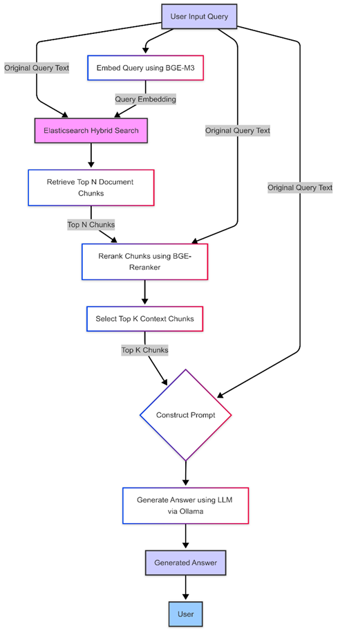
Putting these pieces together – Elasticsearch for flexible hybrid storage and retrieval, open-source embedding and reranking models from Hugging Face, and a powerful open-source LLM served via Ollama – gives us a robust, private, and highly capable AI search solution running entirely on our own infrastructure.

Conclusion: Beyond the Keyword

And there we have it – a journey from the limitations of traditional keyword search (remember those headphones?) to the sophisticated capabilities of modern AI-augmented retrieval. We’ve seen how techniques like semantic search using embeddings remove the barriers between how we think and how we search, allowing for more natural interactions with information. Hybrid approaches offer a pragmatic best-of-both-worlds solution, while Retrieval-Augmented Generation (RAG) takes it a step further, enabling conversational Q&A based on specific document collections.

Perhaps the most exciting takeaway is that building these powerful systems doesn’t necessarily require massive budgets or reliance on external cloud APIs. As we demonstrated with our local setup using Elasticsearch, Hugging Face models, and Ollama, the open-source ecosystem provides potent tools to create private, effective, and customizable AI search solutions.

Whether you’re looking to improve search within your company’s knowledge base, enhance a customer-facing product catalog, or simply explore the cutting edge of information retrieval, the techniques we’ve covered offer a path forward. The era of forcing human language into rigid keyword boxes is fading; the future of search is semantic, contextual, and increasingly intelligent. Hopefully, this series has sparked some ideas for how you can leverage AI-powered search to augment your own information retrieval experiences!